Implementation of a Hyperbolic Vortex Plasma Reactor for the Removal of Micropollutants in Water

Summary

This study presents the methodology for the generation of six different types of plasma discharges within a Hyperbolic Vortex Plasma Reactor for the degradation of micropollutants in water, including pharmaceuticals and per- and polyfluoroalkyl substances (PFAS).

Abstract

The presence of micropollutants in water is an increasingly pressing environmental concern. While some micropollutants are readily biodegradable, others, such as per- and polyfluoroalkyl substances (PFAS), are extremely persistent and resistant to conventional water treatment technologies. Plasma-based treatment has been investigated for water and wastewater decontamination for decades, with recent studies demonstrating its high efficacy in degrading both short- and long-chain PFAS. Here, plasma-based waste treatment is combined with a free surface hyperbolic water vortex, which has an oxygen volumetric mass transfer coefficient exceeding that of similar systems. Various types of plasma discharges can be employed for such applications, each requiring specific power supply configurations and operational strategies. The use of pulsed signals, in particular, presents unique engineering challenges. This study explores the generation and characterization of six different plasma discharge types within a Hyperbolic Vortex Plasma Reactor: pulsed monopolar (negative and positive), pulsed bipolar "flashover," AC and DC arc, and glow discharge. The pulse characteristics of monopolar and bipolar pulsed discharges were analyzed, and their efficiency in PFAS degradation was evaluated. Among the tested configurations, the bipolar flashover discharge exhibited the highest degradation efficiency in a Hyperbolic Vortex Plasma Reactor. However, its practical implementation poses significant engineering challenges, making its utilization challenging on a larger scale.

Introduction

Spiral structures are fundamental to nature, influencing phenomena ranging from the microscopic arrangement of DNA to the vast formations of galaxies^1,2. In fluid dynamics, helical flows exhibit unique properties of mixing, energy transfer, and stability, which can be harnessed for innovative engineering applications³. Inspired by these natural flow patterns, hyperbolic water vortices have been investigated for their potential in enhancing aeration and enabling advanced water treatment technologies^4,5,6,7. This study explores the integration of hyperbolic vortex dynamics with plasma discharge for the degradation of persistent micropollutants, in particular per- and polyfluoroalkyl substances (PFAS).

The initial research into hyperbolic funnels was motivated by their efficiency in aeration, a crucial process in water treatment. These geometrically confined vortices significantly enhance gas-liquid interactions, thereby increasing oxygen transfer rates while minimizing energy consumption⁷. A detailed explanation of the formation and operation of hyperbolic water vortices is provided elsewhere⁶. It soon became clear that the high degree of mixing and surface area increase that resulted in such high aeration capacity could be further utilized for pollutant degradation. Building upon this idea, plasma discharge was introduced into the vortex system, creating a novel hybrid approach for micropollutant removal⁸.

Micropollutants, including pharmaceuticals, pesticides, and PFAS, pose significant environmental and public health challenges due to their persistence and resistance to conventional water treatment methods⁹. Among these, PFAS-commonly referred to as "forever chemicals"-are particularly problematic due to their strong carbon-fluorine bonds, which confer extreme stability and bioaccumulative potential^10,11.

A wide range of technologies has been developed to address PFAS contamination, including adsorption using activated carbon^12,13 and membrane separation¹⁴. While effective at capturing PFAS, these methods are non-destructive and generate secondary waste streams. Activated carbon becomes costly due to frequent regeneration needs-especially at high PFAS loads-and competes with co-contaminants, while membrane systems concentrate PFAS into waste brines requiring further treatment.

Advanced oxidation processes (AOPs) such as electrochemical oxidation, ozonation, UV-based systems, and supercritical water oxidation aim to degrade PFAS rather than separate them^15,16. However, they often suffer from high energy demands, poor selectivity (especially for short-chain PFAS), and the generation of harmful byproducts or incomplete degradation.

Plasma-based technologies have recently gained attention as a promising destructive method, offering rapid PFAS degradation across chain lengths^17,18,19,20. However, most studies report reduced performance on short-chain PFAS, which are frequently generated as intermediate byproducts during the treatment process. Additionally, plasma treatment alone can be energy-intensive and difficult to scale.

Various types of plasma discharge have been explored for water treatment applications. These include direct current (DC) glow and arc discharges, alternating current (AC) discharges, pulsed corona discharge, dielectric barrier discharge (DBD), and gliding arc discharge^{8,21,22,23,24}. Each type of plasma discharge exhibits distinct characteristics in reactive species generation, energy distribution, and pollutant degradation pathways. While glow discharge operates at lower temperatures and provides uniform ionization, arc discharge delivers intense localized heating, making it effective for breaking down persistent organic pollutants^25,26,27. Pulsed discharges, such as monopolar and bipolar pulsed plasma, are characterized by their high-energy density and the generation of transient reactive species, which contribute to enhanced efficiency of micropollutant degradation at moderate energy requirements⁸.

This study demonstrates a method for generating and operating six different types of plasma discharges within a Hyperbolic Vortex Plasma Reactor: (i) pulsed monopolar negative, (ii) pulsed monopolar positive, (iii) pulsed bipolar "flashover" , (iv) AC arc, (v) DC arc, and (vi) glow discharge. Each of these discharge modes has unique interactions with the hyperbolic vortex, influencing the generation of reactive oxygen and nitrogen species (RONS), ultraviolet radiation, shockwaves, energetic electrons, and solvated electrons, all of which contribute to pollutant degradation. The electrode configurations for each plasma discharge type utilized in the experiments are depicted in Figure 1. The integration of such plasma discharge modes with vortex-induced mixing enables enhanced mass transfer and improved contact between contaminants and reactive species, resulting in more effective degradation of micropollutants.

As demonstrated in^28,29, the addition of a cationic surfactant further enhances degradation efficiency by promoting the transport of PFAS molecules to the plasma-water interface, where the most intense reactive processes take place. The results indicate that this system achieves near-complete degradation of PFAS while maintaining operational feasibility.

In addition, as demonstrated elsewhere³⁰, PFAS-contaminated samples treated in a Hyperbolic Vortex Plasma Reactor under an air atmosphere exhibited no increase cytotoxicity or genotoxicity. These findings further support the potential of this technology as a promising approach to PFAS removal.

The implications of this research extend beyond PFAS degradation. The combination of Hyperbolic Vortex Induced Mixing and plasma treatment offers a scalable and adaptable solution for various water treatment challenges, from organic contaminant removal to enhanced oxygenation. Future studies will focus on optimizing reactor configurations, investigating the fate of degradation byproducts, and evaluating long-term system performance in real-world applications.

By combining nature-inspired fluid dynamics with advanced plasma chemistry, this study paves the way for more sustainable and effective water treatment technologies that address critical environmental issues while reducing energy and resource consumption.

Protocol

1. General recommendations

1. Prior to handling the experimental setup, discharge any accumulated static charge by touching conductive parts with a grounding stick.
2. Inspect all hydraulic and electrical connections of the setup for integrity and proper functionality.
3. Initiate the pumps at a low flow rate (80 L·h^-1) using clean water and verify the absence of leakages.
4. Ensure that the reactor is free from gas leaks by purging it with compressed air at 1 atm and applying a soap-water solution to all connections.
   NOTE: If bubbles appear after performing step 1.4, this indicates a gas leak that must be identified and sealed before treatment.

2. Experimental setup

1. Hyperbolic vortex plasma setup (Figure 2)
   1. Discharge all metallic components by touching them with a grounding stick.
      NOTE: If a residual charge is present after working with high voltage, a visible and audible spark will occur between the grounding stick and the charged component.
   2. Activate the Dräger sensor (12 in Figure 2), by pressing and holding the OK button for three seconds to enable detection of ozone, nitrite, and oxygen generated by the plasma. Place the sensor inside the right cabinet to check for potential gas leaks.
   3. Connect the water reservoir (14 in Figure 2) containing deionized water to the setup via the designated hose line.
   4. Start the primary pump by pressing the play button, to introduce water into the hyperbolic funnel, ensuring a flow rate of 85 L·h^-1, that slightly exceeds the threshold required for formation of desirable vortex⁶.
      NOTE: At higher flow rates, the water level in the reactor may rise slightly above the optimal level required for stable operation.
   5. Start the secondary pump by pressing the play button, ensuring a flow rate of 10 L·h^-1 to extract water from the upper section of the hyperbolic funnel, thereby stabilizing the water level and maintaining a constant distance between the electrodes and the water surface.
      NOTE: Using both the primary and secondary pumps ensures a stable water level in the reactor. Operating only the primary pump may lead to fluctuations in the water level.
   6. Once a stable vortex is achieved and no leaks are detected, replace the clean water with the experimental sample and repeat steps 2.1.3 and 2.1.4.
   7. If necessary, fine-tune the electrode-to-water distance to optimize plasma formation.
   8. Purge the reactor with a low flow of compressed air (0.1 atm) to stabilize the internal atmosphere and ensure optimal plasma discharge conditions³¹.
   9. If using a cationic surfactant, connect an auxiliary reservoir containing the surfactant solution and introduce it via a dosing pump at the desired concentration before the reactor inlet.

3. Different types of plasma discharges

1. DC arc discharge
   1. Utilize the electrical circuit depicted in Figure 3A.
   2. Connect the positive and negative high-voltage outputs from the bridge rectifier to the electrodes positioned above the water vortex surface.
      NOTE: If working with a single polarity (either positive or negative), ground the respective terminal and operate exclusively with the preferred polarity.
   3. Connect the variac to the 230 V AC power outlet and disengage the red safety switch to enable high voltage.
   4. Ignite the plasma discharge by gradually increasing the voltage (0 V to 250 V) using the variac.
2. AC arc discharge
   1. Utilize the electrical circuit depicted in Figure 3B.
   2. Connect both high-voltage outputs to the electrodes positioned above the water vortex surface.
      NOTE: If operating with a single output, ground the respective terminal.
   3. Connect variac to the 230 V AC power outlet and disengage the red safety switch to enable high voltage.
   4. Ignite the plasma discharge by gradually increasing the voltage (0 V to 250 V) using the variac.
3. Glow discharge in helium atmosphere
   1. Utilize the electrical circuit depicted in Figure 4.
      NOTE: Different electrical circuits can be employed depending on the specific glow discharge requirements (Figure 3, Figure 4, Figure 5, and Figure 6).
   2. Connect the high-voltage outputs to the electrodes positioned above the water vortex surface.
      NOTE: The glow discharge forms between electrodes of opposite polarity. Adjusting the number and placement of electrodes modifies the discharge topology.
   3. Connect variac to the 230 V AC power outlet and disengage the red safety switch to enable high voltage.
   4. Introduce helium at the preferred flow rate by opening a gas valve.
      NOTE: Allow sufficient time for helium to replace the ambient air. The glow discharge color transitions from purple to white as helium concentration increases. Higher flow rates of helium gas enhance discharge brightness.
   5. Ignite the plasma discharge by gradually increasing the voltage from 0 V using the variac until electrical breakdown occurs between the electrodes and the plasma transitions from glow discharge to arc discharge.
      NOTE: Excessive voltage may transform the glow discharge into a pulsed arc discharge due to capacitor effects in the circuit.
4. Bipolar "flashover" pulsed discharge
   1. Utilize the electrical circuit depicted in Figure 4.
   2. Connect the high-voltage outputs to the electrodes positioned above the water vortex surface.
      NOTE: The circuit in Figure 4 allows for flexible electrode configuration. In this study, 16 electrodes were utilized.
   3. Connect variac to the 230 V AC power outlet and disengage the red safety switch to enable high voltage.
   4. Ignite the plasma discharge by gradually increasing the voltage (0 V to 250 V) using the variac.
5. Monopolar positive and negative pulsed streamer discharges
   1. Utilize the electrical circuit depicted in Figure 5 or Figure 6 for positive or negative discharge, respectively.
   2. Connect the respective high-voltage output (positive or negative) to the electrodes positioned above the water vortex surface.
   3. Connect the opposite terminal to a spark gap and ground the other end.
      NOTE: Alternatively, the spark gap can be grounded via an electrode submerged in the grounded water of the reactor.
   4. Purge the spark gap with compressed air (0.5-1 atm) by opening the gas valve and adjusting the flow to ensure a stable internal atmosphere and maintain consistent temperature.
      NOTE: Variations in gas composition, temperature, pressure and electrode spacing within the spark gap influence plasma characteristics.
   5. Connect variac to the 230 V AC power outlet and disengage the red safety switch to enable high voltage.
   6. Ignite the plasma discharge by gradually increasing the voltage (0 V to 250 V) using the variac.
6. Experiment termination
   1. Cease high voltage operation by reducing the variac voltage, switching off the power supply, and engaging the safety switch.
   2. If applicable, stop the dosing pump for the cationic surfactant.
   3. Close all gas valves for helium and compressed air if they were used.
   4. Verify the grounding of all metallic components by touching them with a grounding stick.
   5. Reverse pump flow direction to transfer treated samples back to the water reservoir.
   6. Rinse the setup by circulating clean water and/or an organic solvent through the system.
   7. Properly collect and dispose of waste, ensuring compliance with safety regulations for hazardous substances.
   8. Conduct a final inspection to confirm that all components are powered off, no leaks are present, and the setup is secure for subsequent use.

Results

The electric circuits illustrated in Figure 3, Figure 4, Figure 5, and Figure 6 operate as follows: A variac (V), connected to the 230 V AC grid, regulates the input voltage and supplies it to a neon transformer (T), which steps up the voltage to high-voltage AC. This high-voltage AC is then converted to high-voltage DC by a bridge rectifier composed of diodes (D₁-D₄). The resulting DC signal charges the capacitors (C_x), and the current is distributed across multiple branches through additional diodes (D_x). Bleeder resistors (R_x) are included to ensure a gradual discharge of the capacitors after the system is shut down. In the monopolar discharge configuration, a spark gap (SG) is used to interconnect the grounded terminals of capacitors on the inactive polarity side.

Figure 7 illustrates a comparative analysis of the current and voltage pulse profiles for monopolar positive, monopolar negative, and bipolar flashover plasma discharges. The pulse duration of the flashover discharge was approximately two orders of magnitude shorter than that of the monopolar pulses (0.6 µs vs. 60 µs, respectively). Moreover, the peak current of the flashover discharge (3.4 A) was significantly higher compared to the monopolar positive (60 mA) and negative (30 mA) pulses. In the case of monopolar pulses, plasma filaments propagate along the water surface. Conversely, for the flashover discharge, a plasma channel is established through the gas-water interface between the cathode and anode. When plasma filaments of opposite polarities converge at the water surface, they create a low-impedance conductive plasma channel, enhancing the mobility of charged particles. This reduction in impedance is associated with the shorter pulse duration observed in the flashover discharge regime.

Figure 8 presents the LTspice³² simulation of the potential difference during capacitor charging and rapid discharge, corresponding to the electrical circuits shown in Figure 4, Figure 5, and Figure 6. The simulation illustrates capacitor charging through AC-to-DC conversion via a high-voltage bridge rectifier. As plasma discharge cannot be directly simulated in LTspice, a voltage-controlled switch was implemented to emulate breakdown. Upon triggering, a rapid voltage drop occurs. While the detailed shape of the discharge pulse could not be modeled-due to its dependence on factors such as pressure, temperature, humidity, electrode gap, and water conductivity-the simulation clearly demonstrates the functionality of the proposed circuits and their ability to generate pulsed signals with various polarity configurations.

Figure 9 plots the energy per pulse and power consumption for the three types of discharges. The power input for the positive monopolar discharge was measured at 1.8 W, the negative monopolar discharge at 1.6 W, and the flashover discharge at 1.2 W. Therefore, at a given plasma power, the plasma treatment duration directly corresponds to the total energy input. A detailed description of the energy measurement methodology can be found in⁸.

Figure 10 depicts the changes in water chemistry after 75 min of plasma treatment in an air atmosphere using the three discharge types. Key parameters analysed include pH, oxidation-reduction potential (ORP), electrical conductivity (EC), and the concentrations of reactive oxygen (hydrogen peroxide H₂O₂) and nitrogen species (nitrite NO₂^- and nitrate NO₃^-). Among the three discharges, the flashover discharge induced the most pronounced chemical changes and the highest RONS production. Despite requiring the lowest power input (1.2 W, Figure 9), the flashover discharge exhibited the highest treatment efficiency. This can be attributed to its short pulse duration, which prevents streamers from transitioning into hot arcs with significant ohmic dissipation, thereby enhancing ionization probability and reactive species generation.

Additionally, the flashover discharge establishes a plasma channel between two oppositely charged electrodes positioned at the plasma-water interface, extending approximately 5 cm in length. This configuration significantly increases the plasma-water interaction area compared to monopolar pulses, thereby enhancing reactive species production and facilitating more effective treatment of the liquid phase.

All PFAS samples were analyzed by liquid chromatography-mass spectrometry. A column (1.8 µm, 50 × 2.1 mm) was used for the analysis. To ensure sample stability, they were diluted 1:1 with methanol, and 1 mL of the diluted sample was transferred into a plastic cation vial. Defluorination was assessed by measuring the concentration of free fluoride ions in the water samples using a combination fluoride electrode.

Figure 11 discusses the degradation of perfluorooctanesulfonic acid (PFOS) over time for initial concentrations of 14 µg·L⁻¹ ± 5% and 240 µg·L⁻¹ ± 5%. The flashover discharge demonstrated the highest PFOS degradation efficiency while requiring the lowest energy input. Consequently, subsequent experiments were conducted exclusively with the flashover discharge to optimize treatment performance.

Figure 12 demonstrates the degradation of a PFAS matrix, consisting of molecules of varying chain lengths, along with detected degradation byproducts. While long-chain PFAS exhibited degradation efficiencies exceeding 92% after 75 min of treatment, shorter-chain PFAS showed significantly lower degradation rates. Furthermore, short-chain PFAS compounds (perfluorohexanoic acid (PFHxA), perfluoropentanoic acid (PFPeA), and perfluorobutanoic acid (PFBA)) emerged as degradation byproducts of longer-chain molecules, with no observable degradation of these shorter species. This can be explained by the distinct physicochemical properties of PFAS. Long-chain PFAS, possessing strong surfactant properties, tend to accumulate at the gas-liquid interface or adhere to surfaces, facilitating interaction with plasma-generated energetic species. In contrast, short-chain PFAS exhibit greater hydrophilicity and tend to remain dispersed in the bulk solution, limiting their direct exposure to plasma³³. As previously reported³¹, the primary degradation pathway for PFAS in plasma systems involves interactions with plasma-generated reactive species such as electrons, ions, hydroxyl radicals and solvated electrons. Due to their short lifetimes, these species are primarily confined to the air-water interface. Consequently, long-chain PFAS, which preferentially accumulate at the surface, undergo more efficient degradation, whereas short-chain PFAS, which remain dissolved in the bulk solution, are less affected. In the same study, PFAS degradation was evaluated both with and without air purging. The concentration of reactive species was significantly higher in the non-purged system, which slightly enhanced the degradation of short-chain PFAS. However, this also led to increased energy dissipation within the plasma zone, resulting in reduced degradation efficiency for long-chain PFAS.

Most PFAS molecules function as anionic surfactants due to their negatively charged terminal functional groups (like e.g. RCOO^-, RSO₃^-)³³. To enhance the degradation efficiency of short-chain PFAS, which exhibit weaker surfactant properties, a cationic surfactant, Hyamine 1622, was added at a flow rate of 4 µM·min⁻¹. This surfactant interacts with the negatively charged PFAS headgroups, forming ion pairs that facilitate transport to the plasma-water interface, thereby significantly improving degradation efficiency. The primary degradation pathway is proposed to involve interactions between PFAS-Hyamine complexes and plasma-generated electrons and ions³¹.

Figure 13 shows the degradation of the same PFAS matrix as in Figure 12, but with the addition of the surfactant. A comparison of Figures 12 and 13 clearly demonstrates that surfactant dosing substantially improves degradation efficiency for both long-chain and short-chain PFAS molecules. After 10 min of treatment, long-chain PFAS degradation exceeded 90%, reaching over 97% after 75 min. Similar to the results observed in the absence of surfactant, short-chain PFAS require a longer degradation time, partly due to their formation as degradation byproducts of longer-chain compounds. However, the introduction of Hyamine 1622 significantly enhances the degradation of short-chain PFAS. Specifically, PFBA treatment results improved from 19% recovery to 53% degradation, while PFBS degradation increased from 22% to 95% after 75 min of treatment. PFAS concentrations prior to treatment and following treatment, both with and without surfactant dosing, are presented in Table 1.

Furthermore, degradation byproducts, including PFHxA and PFPeA, were detected. However, unlike in the previous experiments, their concentrations declined after 20 min for PFHxA and 30 min for PFPeA. After 75 min of treatment, their concentrations approached the detection limit, indicating progressive chain-shortening of PFAS degradation intermediates. Additionally, defluorination efficiency improved from 48% to 82% (Figure 14), further supporting the observed degradation trends and suggesting a high degree of PFAS mineralization.

Additionally, PFAS-contaminated groundwater samples were treated with and without surfactant addition for 75 min (Figure 15). The initial PFAS concentrations are presented in Table 2. These samples were collected from shallow aquifers in the Netherlands, however, due to confidentiality agreements, the exact locations cannot be disclosed. Compared to the results shown in Figures 12 and 13, the overall degradation efficiency was lower in both cases-with and without surfactant dosing. Notably, the degradation of short-chain PFAS containing carboxylic functional groups, such as PFPeA and PFBA, remained limited even with surfactant dosing, reaching only 40% and 2% removal, respectively. This reduced efficiency is likely due to the high concentrations of competing ions present in the groundwater (Table 3), which may hinder the formation of PFAS-Hyamine complexes and thus limit their degradation. These findings suggest that highly contaminated samples may benefit from pretreatment to reduce ion concentrations or may require extended treatment durations. Remarkably, a substantial decrease in both total organic and inorganic carbon was observed in all cases (Table 3), indicating that plasma treatment is capable of degrading not only PFAS but also a broad range of other substances in solution-highlighting its potential as a versatile water treatment technology.

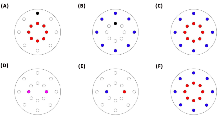
Figure 1: Electrode configurations for various plasma discharge types. Red circles denote electrodes with positive polarity, blue circles indicate electrodes with negative polarity, purple circles represent electrodes connected to high-voltage AC, and black circles correspond to grounded electrodes due to their connection with grounded water in the reactor. (A) monopolar positive discharge, (B) monopolar negative discharge, (C) bipolar flashover discharge, (D) AC arc discharge, (E) DC arc discharge, and (F) glow discharge. Please click here to view a larger version of this figure.

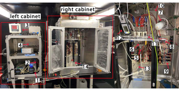
Figure 2: Photo of the Hyperbolic Vortex Plasma setup: 1. Peristaltic pumps; 2. pH, oxidation reduction potential (ORP), and electrical conductivity (EC) probes; 3. Transmitter; 4. BNC connectors for voltage and current signal measurement; 5. Hyperbolic funnel; 6. Stainless steel electrodes; 7. High-voltage probe; 8. Current transformer; 9. Custom made electric circuit; 10. Neon-transformer; 11. Funnel lid with installed electrodes, ventilation, and gas line connections; 12. Gas detector; 13. Grounded water inlets and outlets to the cabinet; 14. Water reservoir. Please click here to view a larger version of this figure.

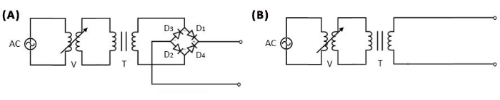
Figure 3: Electric circuit diagram of the high voltage power supply used for experiments. (A) DC arc plasma discharge, (B) AC arc plasma discharge. Please click here to view a larger version of this figure.

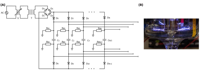
Figure 4: Electric circuit diagram of the high voltage power supply used for the experiments with bipolar flashover and glow discharges. (A) Electric circuit, (B) photograph of the bipolar flashover plasma discharge in operation. Please click here to view a larger version of this figure.

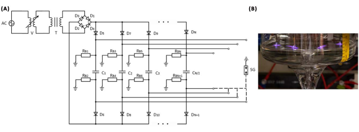
Figure 5: Electrical circuit diagram of the high-voltage power supply used for experiments with monopolar positive discharge. (A) Electric circuit, (B) photograph of the monopolar positive plasma discharge in operation. Please click here to view a larger version of this figure.

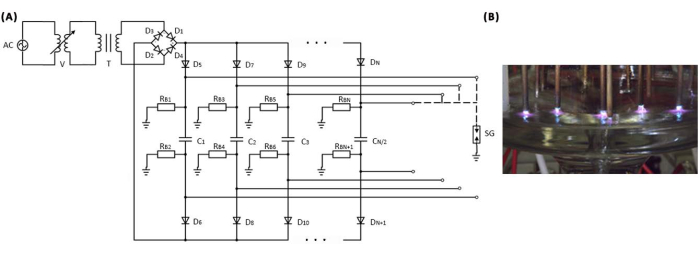
Figure 6: Electric circuit diagram of the high voltage power supply used for experiments with monopolar negative discharge. (A) Electric circuit, (B) photograph of the monopolar negative plasma discharge in operation. Please click here to view a larger version of this figure.

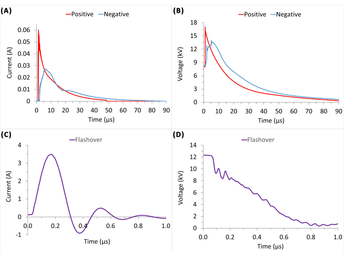
Figure 7: Pulse characteristics of current and voltage. (A,B) For positive and negative monopolar discharges, (C,D) for bipolar flashover discharge. Please click here to view a larger version of this figure.

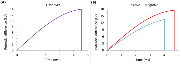
Figure 8: Simulation of potential difference during capacitor charging and rapid discharge in LTspice. (A) For flashover discharge and (B) for positive and negative monopolar discharges. Please click here to view a larger version of this figure.

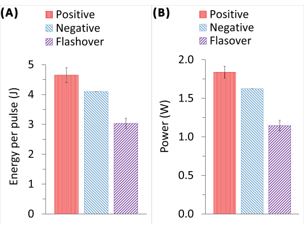
Figure 9: Energy characteristics for three different types of bi- and monopolar discharges: bipolar flashover, positive monopolar, and negative monopolar. (A) Energy per pulse, (B) plasma power. Please click here to view a larger version of this figure.

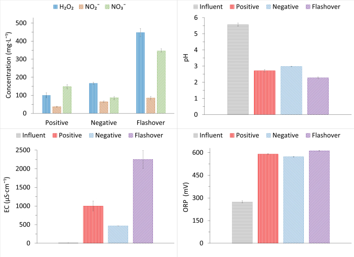
Figure 10: Change in the water chemical properties, pH, EC, ORP, production of reactive oxygen (H₂O₂), and nitrogen species (NO₂⁻ and NO₃⁻), after 75 min of treatment for three different types of bi- and monopolar discharges: bipolar flashover, positive monopolar, and negative monopolar. Please click here to view a larger version of this figure.

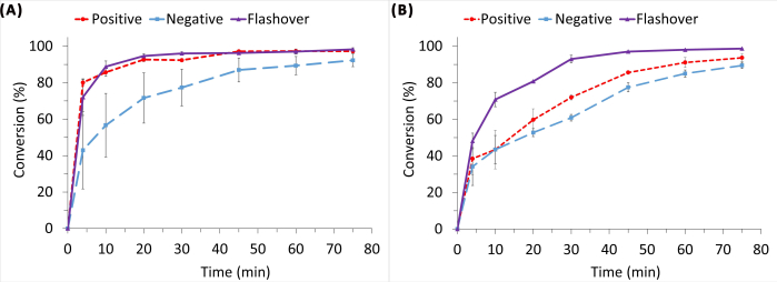
Figure 11: Degradation of PFOS over time at different concentrations. The results compare three discharge modes: bipolar flashover, positive monopolar, and negative monopolar discharges. (A) 14 µg·L⁻¹ ± 5%, (B) 240 µg·L⁻¹ ± 5%. Please click here to view a larger version of this figure.

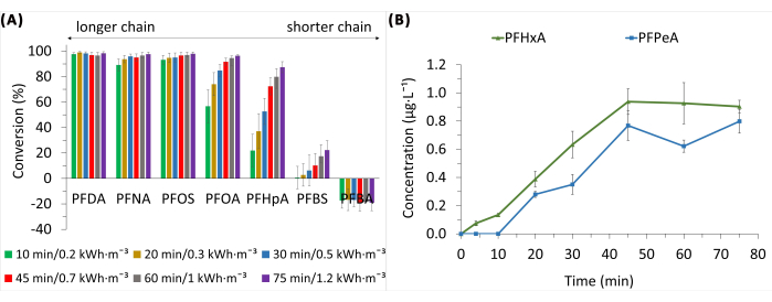
Figure 12: Conversion of the PFAS matrix over time in artificial effluent. Negative values indicate PFAS recovery. (A) PFAS matrix conversion, (B) identified degradation byproducts. Please click here to view a larger version of this figure.

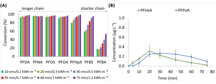
Figure 13: Conversion of the PFAS matrix over time in artificial effluent under constant dosing of Hyamine 1622. (A) PFAS matrix conversion, (B) identified degradation byproducts. Please click here to view a larger version of this figure.

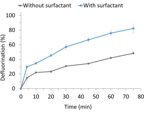
Figure 14: PFAS matrix defluorination in artificial effluent over time under air plasma discharge with and without constant Hyamine 1622 surfactant dosing. Please click here to view a larger version of this figure.

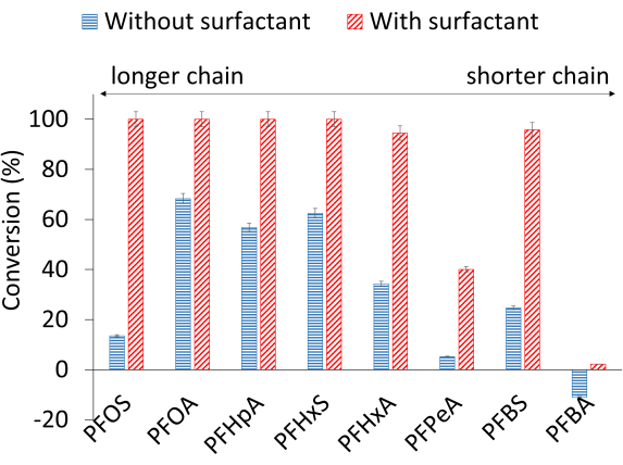
Figure 15: PFAS conversion in contaminated groundwater after 75 min of treatment with energy input of 1.2 kWh·m^-3 with and without Hyamine 1622 dosing. A negative value indicates PFAS recovery. Please click here to view a larger version of this figure.

Name	Formula	Initial concentration (µg·L-1)	Final concentration without surfactant dosing (µg·L-1)	Final concentration with surfactant dosing (µg·L-1)
PFDA	C10HF19O2	6.2	0.12	0.12
PFNA	C9HF17O2	11.8	0.41	0.47
PFOS	C8HF17O3S	8.7	0.65	0.22
PFOA	C8HF15O2	16.3	1.20	0.52
PFHpA	C7HF13O2	13.9	3.94	0.17
PFBS	C4HF9O3S	19.1	16.37	0.90
PFBA	C4HF7O2	10.3	12.69	4.81

Table 1: Concentrations of PFAS compounds spiked into artificial effluents before and after treatment, with and without Hyamine 1622 dosing.

Name	Formula	Initial concentration / µg·L-1	Final concentration without surfactant dosing (µg·L-1)	Final concentration with surfactant dosing (µg·L-1)
PFOS	C8HF17O3S	5.0	4.3	<0.03
PFOA	C8HF15O2	2.4	0.8	<0.02
PFHpA	C7HF13O2	0.9	0.4	<0.05
PFHxS	C6HF13O3S	0.6	0.2	<0.05
PFHxA	C6HF11O2	5.5	3.6	0.3
PFPeA	C5HF9O2	2.3	2.2	1.4
PFBS	C4HF9O3S	23.8	17.9	1
PFBA	C4HF7O2	2.7	3	2.6

Table 2: Concentrations of PFAS compounds in groundwater before and after treatment, with and without Hyamine 1622 dosing.

Substance	Without surfactant		With surfactant
	0 min	75 min	0 min	75 min
Inorganic Carbon	562	475	641	480
Total Organic Carbon	252	226	257	221
Sulfate	396	426	420	442
Chloride	2000	2160	2000	2160
Sodium	1692	1756	1660	1788
Potassium	552	578	532	588
Magnesium	133	122	128	117

Table 3: Changes in water content of some substances in mg·L^-1 in groundwater before and after treatment with and without surfactant dosing.

Discussion

Before initiating experiments, all electrical connections must be thoroughly inspected. Prior to interacting with high-voltage components, a grounding stick should be used to discharge any residual charge in the circuit. These comprehensive safety measures must be implemented to mitigate the risk of accidental electric shocks, even in cases of procedural oversight (door switches, bleeder resistor connected to the capacitors, etc.), because high voltage capacitors can recharge due to memory effect, atmospheric static electricity or cosmic radiation. Their order of magnitude stored energy for these experiments typically is 10^-1-10¹ J, being hazardous to even lethal. Therefore steps 1.1 and 2.1.1 are critical for ensuring safe operation of the system. Before powering the system, the setup should be checked for reactor gaseous and liquid phase leakages. Plasma-generated gases contain reactive species that may pose inhalation hazards, making steps 1.4 and 2.1.2 especially important. All inlets and outlets of the operational chamber must be grounded. The reactor enclosure should be constructed from metal and properly grounded to ensure safe operation. Additionally, verifying the absence of water leaks is essential, as PFAS compounds are classified as CMR substances and must not be allowed to contaminate the laboratory environment. Therefore, particular attention should be paid to step 1.3 prior to initiating the experiment.

In this study, the highest performance was achieved with flashover discharges. This discharge mode resulted in greater RONS production (Figure 10) and higher PFOS degradation (Figure 11) while requiring less power than the other tested discharge types (Figure 9). Although flashover discharges demonstrated superior performance, their implementation presents challenges due to the requirement of two oppositely charged channels connected to the same capacitor. Scaling up this approach necessitates a more powerful power supply. In our current setup, a transformer converts main-voltage AC (up to 220 V) to high-voltage AC (up to 10 kV), which is then rectified into DC using diodes. While the resulting DC signal closely approximates an ideal DC waveform, minor fluctuations remain³⁴. Our circuit design provides operational flexibility across multiple regimes. However, large-scale applications will require high-voltage DC power supplies, which typically operate with a single polarity and a single high-voltage output, restricting the ability to work with multiple polarities simultaneously.

AC and DC arc discharges were not tested for micropollutant degradation due to their significantly higher energy consumption, which would render their industrial application economically unfeasible, particularly in the case of DC plasma. In a previous study⁸ it was demonstrated that increasing the plasma-liquid interfacial area enhances RONS generation for the same energy input, thereby improving micropollutant degradation efficiency. In our electrical circuits (Figure 3A, Figure 4, Figure 5, and Figure 6), diodes convert AC power into DC for charging the capacitors, their stored energy then is distributed over the electrode geometries to generate multiple pulsed power plasma discharges.

At atmospheric pressure and standard conditions, a stable glow discharge can only be sustained using noble gases with high ionization energies, such as helium (first ionization energy 24.6 eV) or neon (first ionization energy 21.6 eV)³⁵. Argon, with a first ionization energy of 15.8 eV³⁵, does not support stable glow discharge under these conditions. However, glow discharge can still be generated in air through the application of an external magnetic field for plasma stabilization³⁶. The high cost of noble gas usage made glow discharge unsuitable for micropollutant degradation in this study.

As discussed in the introduction, conventional treatment methods such as adsorption, membrane filtration, and advanced oxidation processes face significant limitations in effectively addressing PFAS contamination. Plasma discharge presents a promising alternative for PFAS degradation, with reported energy consumption ranging from several kWh·m^-3 to over 1000 kWh·m^-3, depending on factors such as micropollutant concentration, sample composition, and plasma parameters^{29,37,38,39,40,41}. However, short-chain PFAS remain particularly resistant to degradation, and shorter-chain byproducts, such as PFBA, have been identified as intermediates in the breakdown of longer-chain PFAS.

The novelty of our work lies in combining a Hyperbolic Vortex Plasma Reactor with cationic surfactant Hyamine 1622 dosing, significantly improving degradation rates, including for short-chain PFAS (Figure 13). This reactor design increases the plasma-liquid interfacial area and facilitates enhanced mixing through the water vortex. In 75 min of treatment at a moderate energy input of 1.2 kWh·m^-3, our system achieves 95-100% degradation of most PFAS (except PFBA, which still shows 53% removal). These results outperform many plasma-only studies and demonstrate that our approach can achieve deep PFAS mineralization under relatively low energy input. However, this study was conducted at the laboratory scale. To enhance its practical application, scaling up is required, including modifications to reactor geometry-specifically, expanding the top cylindrical section-to increase treated water volume and accommodate additional electrodes. These modifications would enhance plasma-water interaction and improve treatment efficiency. While the reactor's electrical design allows for straightforward scaling, increasing operational power demands more robust power supplies and improved safety measures to ensure stable and efficient performance on a larger scale. Scaling up the system will necessitate an increase in power supply and capacitor bank size, which introduces significant safety concerns. All electrical components must be carefully arranged and positioned in close proximity to the reactor while remaining inaccessible during operation. To ensure safe discharge, each capacitor must be individually grounded after use, requiring dedicated grounding switches, as they cannot be interconnected and must be isolated from one another with diodes for direct current separation. Additionally, higher power levels will generate stronger electromagnetic fields that could interfere with nearby instrumentation. Therefore, both the reactor and surrounding equipment should be properly shielded, preferably within a Faraday cage. Precise control of the water vortex is essential, as plasma discharge performance is highly sensitive to flow conditions and funnel geometry. This necessitates a well-programmed hydraulic control system. Furthermore, the reactor must be adequately insulated, connected to a ventilation system, and equipped with a gas inlet for purging. If high concentrations of volatile fluorinated byproducts, such as hydrogen fluoride, are expected, supplementary gas treatment steps should be implemented. These may include dry or wet scrubbing systems^42,43, or the application of calcium-based sorbents⁴⁴.

The energy consumption of the pilot-scale reactor could potentially be reduced through the addition of surfactants, which concentrate PFAS at the air-water interface. By decreasing the surface-to-volume ratio, PFAS compounds become more localized at the interface, allowing the plasma to interact with a higher concentration of target compounds per unit area, thereby increasing degradation efficiency per discharge. However, increasing the overall water volume may extend the required treatment duration, potentially offsetting the energy savings. Utilizing a high-voltage, high-power DC power supply for capacitor charging enables precise control of energy input, allowing systematic evaluation of different energy regimes for optimization.

Future research will focus on scaling up the technology based on the described operational principles to achieve a treatment capacity of 1 m³·h^-1 for pilot-scale applications. Additionally, a detailed investigation of degradation products is essential, with particular interest in the formation and breakdown of the shortest-chain PFAS, trifluoroacetic acid, as well as other potential transformation products. Further studies will also aim to identify an effective, biodegradable, and cost-efficient cationic surfactant capable of enhancing PFAS degradation through improved formation of surfactant-PFAS complexes.

Materials

List of materials used in this article

Name	Company	Catalog Number	Comments
Bleeder resistors	Tedss	RCR42G206JS	20 MOhm
BNC connectors	AliExpress	N/A	BNC ADAPTER
Capacitor	AnXon	AXCT8GD202K40DB	40 kV 2000 pF
Cationic surfactant	Sigma-Aldrich	51126-1L-F	Hyamine 1622 solution
Column	Agilent	Zorbax Eclipse Plus C18 RRHD	1.8 μm, 50 × 2.1 mm
Current transformer	Magnelab	CT-F0.25-S
Data Logger	Endress+Hauser	CM442	Liquiline
Door switches	QWORK	ME-8104	10A 250VAC
Dosing pump	KNF	1.10 TT.18RC2	FEM
Dräger sensor	Dräger	X-am 5000	O2, O3, NO2
EC sensor	Endress and Hauser	CLS15E	Memosens
Electrodes	AliExpress	N/A	Ceramic Ignition Rod
Fluoride electrode	Mettler Toledo	perfectION
Funnel lid	Custom made	N/A	PVC matetial
Grounding stick	Custom made	N/A
Helium gas	Westfalen	UN 1046	99.999 Vol. % He
High voltage diode	Ebay	FHVP5446	1p 5A 40kV
Highvoltage probe	North Star High Voltage	PVM-5
Hyperbolic funnel	Custom made	N/A	Glass material
LC/MS	Agilent Technologies	6420 Triple Quad LC/MS	Santa Clara, CA, USA
Noen-transformer	F/ART	SBD63HT2X	10000V 18mA
ORP sensor	Endress and Hauser	CPS12D	Memosint
Peristaltic pump	Masterflex L/S	13-200-007	MFLX7771236
PFBA	Sigma-Aldrich	375-22-4	PFAS for experiments
PFBS	Sigma-Aldrich	375-73-5	PFAS for experiments
PFDA	Sigma-Aldrich	335-76-2	PFAS for experiments
PFHpA	Sigma-Aldrich	375-85-9	PFAS for experiments
PFNA	Sigma-Aldrich	375-95-1	PFAS for experiments
PFOA	Sigma-Aldrich	335-67-1	PFAS for experiments
PFOS	Sigma-Aldrich	1763-23-1	PFAS for experiments
pH sensor	Endress and Hauser	CPS11D	Memosens Orbisint
Safety interlock control panel	Custom made	N/A
Spark Gap	Custom made	N/A
Variac	Weltechniek	TDGC2-1K	4a
Water reservoir	Custom made	N/A	Glass material

References

- Tsuji, K., Muller, S. C. Spirals and Vortices in Culture, Nature, and Science. , Springer. Cham. (2019).
- Uchiyama, Y., Zhang, X., Yanase, S. Generation mechanism of Tidally-driven whirlpools at a narrow strait in an estuary. IOP Conf Ser Earth Environ Sci. 945, 012028(2021).
- Johansson, L., Ovesen, M., Hallberg, C. Self-organizing Flow Technology - In Viktor Schauberger's Footsteps. , Institute of Ecological Technology Scientific and Technical Reports, Malmo. (2002).
- Agostinho, L. L. F., et al. Enhanced oxygen volumetric mass transfer in a geometrically constrained vortex. Water. 14 (5), 771(2022).
- Donepudi, T., et al. Numerical analysis of vortex dynamics in hyperbolic funnels using computational fluid dynamics. Phys Fluids. 36 (9), 095171(2024).
- Klymenko, R., et al. Preparation of free-surface hyperbolic water vortices. J Vis Exp. (197), e64516(2023).
- Klymenko, R., et al. Enhanced groundwater aeration with a geometrically constrained vortex. Water. 17 (4), 506(2025).
- Klymenko, R., et al. Characterization of a hyperbolic vortex plasma reactor for the removal of aqueous phase micropollutants. J Phys D Appl Phys. 57, 215204(2024).
- Richardson, S., Kimura, S. Emerging environmental contaminants: challenges facing our next generation and potential engineering solutions. Environ Technol Innov. 8, 40-56 (2017).
- Sharma, S., Shetti, N. P., Basu, S., Nadagouda, M. N., Aminabhavi, T. M. Remediation of per- and polyfluoroalkyls (PFAS) via electrochemical methods. Chem Eng J. 430, 132895(2022).
- Dhore, R., Murthy, G. S. Per/polyfluoroalkyl substances production, applications and environmental impacts. Bioresour Technol. 341, 125808(2021).
- Lobato-Peralta, D. R., et al. Advances in activated carbon modification, surface heteroatom configuration, reactor strategies, and regeneration methods for enhanced wastewater treatment. J Environ Chem Eng. 9 (4), 105626(2021).
- Baghirzade, B. S., et al. Thermal regeneration of spent granular activated carbon presents an opportunity to break the forever PFAS cycle. Environ Sci Technol. 55 (9), 5608-5619 (2021).
- Lee, T., Speth, T. F., Nadagouda, M. N. High-pressure membrane filtration processes for separation of per- and polyfluoroalkyl substances (PFAS). Chem Eng J. 431, 134023(2022).
- Meegoda, J. N., Bezerra de Souza, B., Casarini, M. M., Kewalramani, J. A. A review of PFAS destruction technologies. Int J Environ Res Public Health. 19 (24), 16397(2022).
- Olatunde, O. C., Kuvarega, A. T., Onwudiwe, D. C. Photo enhanced degradation of polyfluoroalkyl and perfluoroalkyl substances. Heliyon. 6 (12), e05614(2020).
- Ajo, P., Preis, S., Vornamo, T., Mänttäri, M., Kallioinen, M., Louhi-Kultanen, M. Hospital wastewater treatment with pilot-scale pulsed corona discharge for removal of pharmaceutical residues. J Environ Chem Eng. 6 (2), 1569-1577 (2018).
- Magureanu, M., Bradu, C., Parvulescu, V. I. Plasma processes for the treatment of water contaminated with harmful organic compounds. J Phys D Appl Phys. 51, 313002(2018).
- Kumar, A., Škoro, N., Gernjak, W., Puač, N. Cold atmospheric plasma technology for removal of organic micropollutants from wastewater-a review. Eur Phys J D. 75, 283(2021).
- Sakudo, A., Yagyu, Y., Onodera, T. Disinfection and sterilization using plasma technology: fundamentals and future perspectives for biological applications. Int J Mol Sci. 20 (20), 5216(2019).
- Mouele, E. S. M., et al. Removal of pharmaceutical residues from water and wastewater using dielectric barrier discharge methods-A review. Int J Environ Res Public Health. 18 (4), 1683(2021).
- Choi, S., Watanabe, T., Liu, T. Discharge characteristics of DC arc water plasma for environmental applications. Plasma Sci Technol. 14, 1097-1101 (2012).
- Gharagozalian, M., Dorranian, D., Ghoranneviss, M. Water treatment by the AC gliding arc air plasma. J Theor Appl Phys. 11, 171-180 (2017).
- Zeghioud, H., Nguyen-Tri, P., Khezami, L., Amrane, A., Assadi, A. A. Review on discharge plasma for water treatment: mechanism, reactor geometries, active species and combined processes. J Water Process Eng. 38, 101664(2020).
- Quarles, C. D., Castro, J., Marcus, R. K. Glow Discharge Mass Spectrometry. Encyclopedia of Spectroscopy and Spectrometry. , Academic Press, Elsevier. (2010).
- Lu, P., Boehm, D., Bourke, P., Cullen, P. J. Achieving reactive species specificity within plasma-activated water through selective generation using air spark and glow discharges. Plasma Process Polym. 14 (8), e1600207(2017).
- Shrestha, R., et al. Treatment of water using Arc discharge plasma in Patan area. Patan Prospect J. 2 (2), 150-163 (2022).
- Singh, R. K., Brown, E., Mededovic, T. S., Holsen, T. M. Treatment of PFAS-containing landfill leachate using an enhanced contact plasma reactor. J Hazard Mater. 408, 124452(2021).
- Singh, R. K., et al. Removal of poly- and per-fluorinated compounds from ion exchange regenerant still bottom samples in a plasma reactor. Environ Sci Technol. 54 (21), 13973-13980 (2020).
- Windisch, M., Klymenko, R., Grießler, H., Kittinger, C. Assessment of cytotoxicity and genotoxicity of plasma-treated perfluorooctanesulfonate containing water using in vitro bioassays. Toxics. 12 (12), 889(2024).
- Klymenko, R., et al. PFAS degradation using a hyperbolic vortex plasma reactor. J Phys D Appl Phys. 58, 175204(2025).
- Ltspice, Analog Devices. , https://www.analog.com/en/resources/design-tools-and-calculators/ltspice-simulator.html (2025).
- Leung, S. C. E., Wanninayake, D., Chen, D., Nguyen, N. -T., Li, Q. Physicochemical properties and interactions of perfluoroalkyl substances (PFAS) - Challenges and opportunities in sensing and remediation. Sci Total Environ. 905, 166764(2023).
- Lee, Y. -S., Chow, M. H. L. Diode Rectifiers. Power Electronics Handbook. , Elsevier. Burlington. (2007).
- NIST Atomic Spectra Database (ASD). , National Institute of Standards and Technology. At At https://physics.nist.gov/PhysRefData/ASD/ionEnergy.html (2024).
- Yu, L. Z., Lan, N. L., Liu, D. W., Pei, L. X. An atmospheric pressure glow discharge in air stabilized by a magnetic field and its application on nitrogen fixation. Plasma ProcessPolym. 19 (12), 2200071(2022).
- Tamanga, S. G., Umlaufb, G., Barzb, J., Ghomi, M. R. Degradation of PFOA solutions and PFAS-contaminated groundwater using atmospheric non-thermal plasma treatment. Water Pract Technol. 19 (7), 2645-2654 (2024).
- Alam, D., et al. Experimental investigations of Per- and Poly-fluoroalkyl substances (PFAS) degradation by non-thermal plasma in aqueous solutions. J Environ Chem Eng. 11 (6), 111588(2023).
- Zhang, H., et al. Removal of per- and polyfluoroalkyl substances from water by plasma treatment: Insights into structural effects and underlying mechanisms. Water Res. 253, 121316(2024).
- Chen, C., et al. Degradation of perfluoroalkyl and polyfluoroalkyl substances (PFAS) in water by use of a nonthermal plasma-ozonation cascade reactor: Role of different processes and reactive species. Chem Eng J. 486, 150218(2024).
- Lewis, A. J., et al. Rapid degradation of PFAS in aqueous solutions by reverse vortex flow gliding arc plasma. Environ Sci Water Res. Technol. 6 (4), 1044-1057 (2020).
- McIntosh, G. J., Agbenyegah, G. E. K., Hyland, M. M., Metson, J. B. The pivotal role of alumina pore structure in HF capture and fluoride return in aluminum reduction. JOM. 68, 2463-2471 (2016).
- Mukherjee, S., Siddiqi, H., Maiti, P., Parmar, P., Meikap, B. C. A comprehensive analysis of removal of hazardous dust particulates from chemical and process industries off gases by advanced wet scrubbing techniques - A review. J Loss Prev Process Ind. 91, 105406(2024).
- Comparison of sodium and calcium based sorbents for the dry treatment of flue gas from waste-to-energy plants. Zach, B., et al. 2nd International Conference on Energy Production and Management (EQ 2016), , Ancona. (2016).
Reprints and Permissions